Non-Centered Parameterisation in Hierarchical Bayesian Models: Not Just For Univariate Gaussians
What is a Hierarchical Bayesian Model?
Hierarchical Bayesian models assess individual variation (e.g., between people) in a parameter or quantity of interest while simultaneously producing insights about group or population level effects. This type of model is useful because it avoids the need to a) assume the parameter or quantity of interest is identical across the population or b) assume individuals within the same population are completely independent. The hierarchical model recognises that individuals within a population are likely to share certain common characteristics with other members of that population, but also recognises the presence of individual variation within that population.
Suppose we want to examine the impact of weekly working hours on mental health in a particular population, and that we have multilevel data where multiple observations of both weekly working hours and mental health were taken over time for a set of individuals. A hierarchical Bayesian model would allow us to estimate the impact of working hours on mental health for each individual. However, each individual’s estimated effect would be informed not only by that individual’s data, but also in part by the estimated effects from other individual’s in the population. This phenomenon is sometimes referred to as ‘partial pooling’ of information. It means that information about the parameter or quantity of interest (in this case, the effect of working hours on mental health) is shared or ‘pooled’ across individuals in the sample. The ‘partial’ bit means that an individual’s estimate is not completely determined by the information about other individuals’ estimates. The model leaves room for individual variation by estimating unique effects for each individual.
The usefulness of hierarchical Bayesian models is well documented elsewhere (e.g., see here, here, or for work from my own lab see here ). The point of this post is not to further highlight the virtues of these models. The point is to explain one particularly tricky aspects of actually implementing them.
What is a Non-Centered Parameterisation?
To explain what a non-centered parameterisation is and why it’s useful,
let’s start with a simple example. Let’s simulate some multilevel data.
In this example, we’ll assume we have 500 participants who each produce
5 observations of three variables: X1, X2, and Y. In the code below, the
parameters beta0, beta1, beta2, and sigma represent the intercept,
linear effect of X1, linear effect of X2, and the residual error
respectively. We first assign population-level distributions
representing the variation in these parameters across participants. We
then randomly sample the parameter values for each participant based on
the population-level distributions we defined. Finally, we use the
participant-level parameters and the covariates X1 and X2 to randomly
generate response variable Y, before creating a list containing that
data that can be read into stan.
# Set random seed for reproducibility
set.seed(123)

# Simulate data
N <- 2500  # Total number of observations
J <- 500    # Number of participants
n_j <- N / J  # Number of observations per participant

# Generate participant IDs and predictor variables
participant_id <- rep(1:J, each = n_j)
X1 <- rnorm(N, mean = 0, sd = 1)
X2 <- rnorm(N, mean = 0, sd = 1)

# Population parameter values
beta0_mean <- 2.5   # beta0 population mean
beta1_mean <- 1.5   # Effect of X1 population mean
beta2_mean <- -0.2  # Effect of X2 population mean
beta0_sd <- 1.5     # beta0 population SD
beta1_sd <- 1.3     # Effect of X1  population SD
beta2_sd <- 0.7     # Effect of X2 population SD
sigma_mean <- 0.7   # Residual mean
sigma_sd <- 0.3     # Residual SD

# Simulate variability in parameters across participants
beta0 <- rnorm(n = J, mean = beta0_mean, sd = beta0_sd)
beta1 <- rnorm(n = J, mean = beta1_mean, sd = beta1_sd)
beta2 <- rnorm(n = J, mean = beta2_mean, sd = beta2_sd)
sigma <- truncnorm::rtruncnorm(n = J, a = 0, b = Inf, mean = sigma_mean, sd = sigma_sd)

# Generate response variable
Y <- rep(beta0, each = n_j) +
  rep(beta1, each = n_j) * X1 +
  rep(beta2, each = n_j) * X2 +
  rnorm(N, mean = 0, sd = rep(sigma, each = n_j))

# Prepare data for Stan
stan_data <- list(
  N = N,
  J = J,
  X1 = X1,
  X2 = X2,
  Y = Y,
  participant_id = participant_id
)
Now let’s define a hierarchical Bayesian model of this data in stan. What makes the model below hierarchical is that the priors on the participant-level parameters defined in the model section depend on the population-level parameters, which themselves are uncertain and therefore estimated by the model. Information from each participant’s data flows “up the hierarchy” influencing the population-level parameters via the individual-specific parameters. But information about the population parameters in turn flows back down the hierarchy by constraining the individual parameters to values that are more plausible given the distribution of those parameters in the population.
stan_model <- "
data {
  int<lower=0> N;               // Number of observations
  int<lower=0> J;               // Number of participants
  vector[N] X1;                 // Predictor 1
  vector[N] X2;                 // Predictor 2
  vector[N] Y;                  // Response variable
  array[N] int participant_id;  // Participant IDs
}

parameters {
  real beta0_mean;            // Intercept population mean
  real beta1_mean;            // Effect of X1 population mean
  real beta2_mean;            // Effect of X2 population mean
  real<lower=0> beta0_sd;     // Intercept population SD
  real<lower=0> beta1_sd;     // Effect of X1 population SD
  real<lower=0> beta2_sd;     // Effect of X2 population SD
  real<lower=0> sigma_mean;   // Residual mean
  real<lower=0> sigma_sd;     // Residual SD
  vector[J] beta0;            // Participant intercepts
  vector[J] beta1;            // Participant X1 effects
  vector[J] beta2;            // Participant X2 effects
  vector<lower=0>[J] sigma;   // Participant residuals
}

model {
  // Population-level Priors
  beta0_mean ~ normal(0, 5);
  beta1_mean ~ normal(0, 5);
  beta2_mean ~ normal(0, 5);
  beta0_sd ~ normal(0, 2.5);
  beta1_sd ~ normal(0, 2.5);
  beta2_sd ~ normal(0, 2.5);
  sigma_mean ~ normal(0, 2.5);
  sigma_sd ~ normal(0, 2.5);

  // Participant-level Priors
  beta0 ~ normal(beta0_mean,beta0_sd);
  beta1 ~ normal(beta1_mean,beta1_sd);
  beta2 ~ normal(beta2_mean,beta2_sd);
  sigma ~ normal(sigma_mean,sigma_sd);

  // Likelihood
  Y ~ normal(beta0[participant_id] + beta1[participant_id] .* X1 + beta2[participant_id] .* X2, sigma[participant_id]);
}
"
We can fit the model using the code below.
# Compile the model
mod <- cmdstan_model(write_stan_file(stan_model))

# Fit the model
fit <- mod$sample(
  data = stan_data,
  seed = 123,
  chains = 4,
  parallel_chains = 4,
  refresh = 0,
  show_exceptions = FALSE
)
## Running MCMC with 4 parallel chains...
##
## Chain 2 finished in 34.7 seconds.
## Chain 1 finished in 47.3 seconds.
## Chain 3 finished in 48.2 seconds.
## Chain 4 finished in 53.1 seconds.
##
## All 4 chains finished successfully.
## Mean chain execution time: 45.8 seconds.
## Total execution time: 53.2 seconds.

## Warning: 694 of 4000 (17.0%) transitions ended with a divergence.
## See https://mc-stan.org/misc/warnings for details.
As you can see from the message after the model finished, there were a lot of divergent transitions. This means the sampler is having difficulty exploring the posterior distribution effectively. This is common when hierarchical models are specified this way, because the scale of each participant-level parameter depends on another parameter in the model. This dependency can create a posterior geometry that is tricky to sample from efficiently.
This is where the non-centered parameterisation can be helpful1.
It removes this dependency by reparameterising the participant-level
parameters. In the model below, a non-centered parameterisation is
applied to beta0, beta1, and beta2 (sigma is a little more complicated
since it’s bounded at 0. We’ll get to that next). As you can see, we now
estimate z-scores for these three parameters and then in the
transformed parameters block unstandardise the parameter via an
inverse-z transform.
stan_model_nc <- "
data {
  int<lower=0> N;               // Number of observations
  int<lower=0> J;               // Number of participants
  vector[N] X1;                 // Predictor 1
  vector[N] X2;                 // Predictor 2
  vector[N] Y;                  // Response variable
  array[N] int participant_id;  // Participant IDs
}

parameters {
  real beta0_mean;            // Intercept population mean
  real beta1_mean;            // Effect of X1 population mean
  real beta2_mean;            // Effect of X2 population mean
  real<lower=0> beta0_sd;     // Intercept population SD
  real<lower=0> beta1_sd;     // Effect of X1 population SD
  real<lower=0> beta2_sd;     // Effect of X2 population SD
  real<lower=0> sigma_mean;   // Residual mean
  real<lower=0> sigma_sd;     // Residual SD
  vector[J] beta0_z;          // Participant intercepts (z-score)
  vector[J] beta1_z;          // Participant X1 effects (z-score)
  vector[J] beta2_z;          // Participant X2 effects (z-score)
  vector<lower=0>[J] sigma;   // Participant residuals
}

transformed parameters {
  vector[J] beta0 = beta0_mean + beta0_sd * beta0_z;
  vector[J] beta1 = beta1_mean + beta1_sd * beta1_z;
  vector[J] beta2 = beta2_mean + beta2_sd * beta2_z;
}

model {
  // Population-level Priors
  beta0_mean ~ normal(0, 5);
  beta1_mean ~ normal(0, 5);
  beta2_mean ~ normal(0, 5);
  beta0_sd ~ normal(0, 2.5);
  beta1_sd ~ normal(0, 2.5);
  beta2_sd ~ normal(0, 2.5);
  sigma_mean ~ normal(0, 2.5);
  sigma_sd ~ normal(0, 2.5);

  // Participant-level Priors
  beta0 ~ std_normal();
  beta1 ~ std_normal();
  beta2 ~ std_normal();
  sigma ~ normal(sigma_mean,sigma_sd);

  // Likelihood
  Y ~ normal(beta0[participant_id] + beta1[participant_id] .* X1 + beta2[participant_id] .* X2, sigma[participant_id]);
}
"

# Compile the model
mod_nc <- cmdstan_model(write_stan_file(stan_model_nc))

# Fit the model
fit_nc <- mod_nc$sample(
  data = stan_data,
  seed = 123,
  chains = 4,
  parallel_chains = 4,
  refresh = 0,
  show_exceptions = FALSE
)
## Running MCMC with 4 parallel chains...
##
## Chain 4 finished in 215.4 seconds.
## Chain 1 finished in 282.4 seconds.
## Chain 3 finished in 355.7 seconds.
## Chain 2 finished in 360.8 seconds.
##
## All 4 chains finished successfully.
## Mean chain execution time: 303.6 seconds.
## Total execution time: 360.9 seconds.

## Warning: 1473 of 4000 (37.0%) transitions ended with a divergence.
## See https://mc-stan.org/misc/warnings for details.

## Warning: 2527 of 4000 (63.0%) transitions hit the maximum treedepth limit of 10.
## See https://mc-stan.org/misc/warnings for details.
We’re still getting a lot of divergences and we’re hitting the maximum
treedepth on many iterations, which suggests that the model still isn’t
sampling efficiently. This is because we still haven’t applied a
non-centered parameterisation to sigma. We’ll do that next.
Non-Centered Parameterisation for Truncated Parameters
What makes beta0, beta1, and beta2 easy to reparameterise is the
fact that these variables can take on any real value. In other words,
they’re not bounded or constrained to a particular range. So we don’t
have to worry about the result of the inverse-z transform satisfying a
particular constraint. But not all parameters are unbounded. A good
example of a bounded parameter is a standard deviation. Standard
deviations must be positive. So when estimating these parameters, a
common approach is to sample from truncated distributions that are
constrained to have a lower bound of 0 (as we have in the models above).
It’s not immediately obvious how the non-centered parameterisation can
be applied to parameters that are bounded.
As it turns out, it’s actually fairly straightfoward. The trick is to
sample the parameter as if it were unconstrained and then convert it via
transformation to impose the appropriate constraints. Let’s assume we
want to apply a non-centered transformation to sigma that accounts for
the constraint that this parameter should be positive. We can do
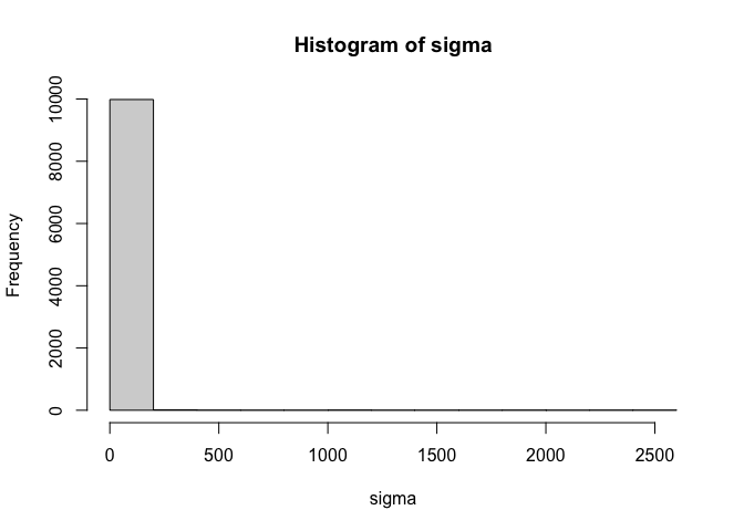
something like what’s done in the R code below. Here, we use the exp()
function to exponentiate the result of the inverse-z transform, which
maps sigma to the positive real numbers. Technically, this
transformation means that sigma is lognormally distributed (in other
words, the log of sigma is normally distributed).
n = 10000                                      #number of samples
sigma_mean = rnorm(n)                          #sample sigma mean
sigma_sd = rtruncnorm(n,a=0)                   #sample sigma sd
sigma_z = rnorm(n)                             #sample sigma z-score
sigma = exp(sigma_mean + sigma_sd * sigma_z)   #unstandardise and convert to positive via exponentiation
hist(sigma)
density(sigma)
##
## Call:
##  density.default(x = sigma)
##
## Data: sigma (10000 obs.);    Bandwidth 'bw' = 0.2097
##
##        x                   y
##  Min.   :  -0.6292   Min.   :0.000000
##  1st Qu.: 636.2959   1st Qu.:0.000000
##  Median :1273.2210   Median :0.000000
##  Mean   :1273.2210   Mean   :0.003456
##  3rd Qu.:1910.1461   3rd Qu.:0.000000
##  Max.   :2547.0712   Max.   :0.815415
Notice in the output above, however, that the resulting distribution of
sigma is heavily skewed. This happens because of the exponential
transformation. Values that are on the high end of the distribution
before the exponentiation get pulled way out when the transformation is
applied. It only takes an untransformed value of 10 to produce a
transformed value of more than 20,000. A prior that is this heavily
skewed can be difficult to sample from. So this transformation may not
help us much. This skew can be alleviated to some extent by placing
different priors on sigma_mean and sigma_sd, but a big part of the
problem is the exponentiation itself.
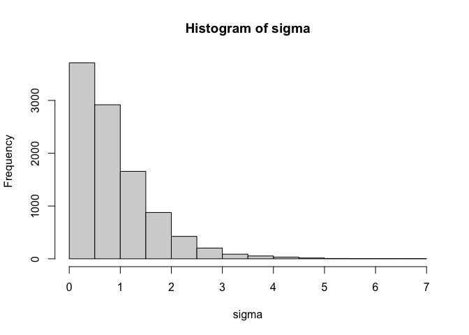
Importantly, there are other transformations that we can apply. One that I particularly like is the softplus transformation $f(x) = log(1+e^x)$. This transformation avoids the heavy skew that can sometimes be created by simply exponentiating. Compare the distribution above with the one below.
n = 10000                                             #number of samples
sigma_mean = rnorm(n)                                 #sample sigma mean
sigma_sd = rtruncnorm(n,a=0)                          #sample sigma sd
sigma_z = rnorm(n)                                    #sample sigma z-score
sigma = log(1+exp(sigma_mean + sigma_sd * sigma_z))   #unstandardise and convert to positive via softplus
hist(sigma)
density(sigma)
##
## Call:
##  density.default(x = sigma)
##
## Data: sigma (10000 obs.);    Bandwidth 'bw' = 0.09291
##
##        x                 y
##  Min.   :-0.2783   Min.   :0.0000049
##  1st Qu.: 1.6020   1st Qu.:0.0009413
##  Median : 3.4822   Median :0.0118323
##  Mean   : 3.4822   Mean   :0.1327000
##  3rd Qu.: 5.3625   3rd Qu.:0.1563247
##  Max.   : 7.2427   Max.   :0.8142086
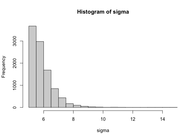
This second distribution is much less skewed and will be easier to sample from. As with the non-centered parameterisation applied to uncontained parameters, you can change the priors on the distribution by modifying the priors on the population parameters. If you want truncate the distribution at a value other than zero, all you need to do is add a constant. The example below truncates the distribution at 5.
n = 10000                                               #number of samples
sigma_mean = rnorm(n)                                   #sample sigma mean
sigma_sd = rtruncnorm(n,a=0)                            #sample sigma sd
sigma_z = rnorm(n)                                      #sample sigma z-score
sigma = 5+log(1+exp(sigma_mean + sigma_sd * sigma_z))   #unstandardise and convert using softplus
hist(sigma)
density(sigma)
##
## Call:
##  density.default(x = sigma)
##
## Data: sigma (10000 obs.);    Bandwidth 'bw' = 0.09155
##
##        x                y
##  Min.   : 4.726   Min.   :0.0000000
##  1st Qu.: 7.354   1st Qu.:0.0000808
##  Median : 9.983   Median :0.0018599
##  Mean   : 9.983   Mean   :0.0949316
##  3rd Qu.:12.611   3rd Qu.:0.0550231
##  Max.   :15.239   Max.   :0.7985695
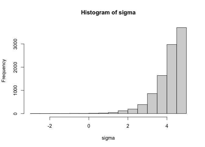
Alternatively, to make the truncation point an upper bound instead of a lower bound, simply multiply the result of the transformation by -1 as in the example below.
n = 10000                                               #number of samples
sigma_mean = rnorm(n)                                   #sample sigma mean
sigma_sd = rtruncnorm(n,a=0)                            #sample sigma sd
sigma_z = rnorm(n)                                      #sample sigma z-score
sigma = 5-log(1+exp(sigma_mean + sigma_sd * sigma_z))   #unstandardise and convert using softplus
hist(sigma)
density(sigma)
##
## Call:
##  density.default(x = sigma)
##
## Data: sigma (10000 obs.);    Bandwidth 'bw' = 0.09081
##
##        x                 y
##  Min.   :-2.9690   Min.   :0.0000059
##  1st Qu.:-0.9087   1st Qu.:0.0014351
##  Median : 1.1516   Median :0.0083201
##  Mean   : 1.1516   Mean   :0.1211043
##  3rd Qu.: 3.2118   3rd Qu.:0.1101382
##  Max.   : 5.2721   Max.   :0.8252533
Here’s a model that uses the softplus transformation to apply a
non-centered parameterisation to the sigma parameter. As you can see,
the process is identical to how we reparameterise the beta parameters
except that the softplus transformation is applied to the parameter
after the inverse-z transform is applied.
stan_model_ncs <- "
data {
  int<lower=0> N;               // Number of observations
  int<lower=0> J;               // Number of participants
  vector[N] X1;                 // Predictor 1
  vector[N] X2;                 // Predictor 2
  vector[N] Y;                  // Response variable
  array[N] int participant_id;  // Participant IDs
}

parameters {
  real beta0_mean;            // Intercept population mean
  real beta1_mean;            // Effect of X1 population mean
  real beta2_mean;            // Effect of X2 population mean
  real<lower=0> beta0_sd;     // Intercept population SD
  real<lower=0> beta1_sd;     // Effect of X1 population SD
  real<lower=0> beta2_sd;     // Effect of X2 population SD
  real sigma_mean;            // Residual population mean (before transformation)
  real<lower=0> sigma_sd;     // Residual population SD (before transformation)
  vector[J] beta0_z;          // Participant intercepts (z-score)
  vector[J] beta1_z;          // Participant X1 effects (z-score)
  vector[J] beta2_z;          // Participant X2 effects (z-score)
  vector[J] sigma_z;          // Participant residuals (z-score, before transformation)
}

transformed parameters {
  vector[J] beta0 = beta0_mean + beta0_sd * beta0_z;
  vector[J] beta1 = beta1_mean + beta1_sd * beta1_z;
  vector[J] beta2 = beta2_mean + beta2_sd * beta2_z;
  vector[J] sigma = log1p_exp(sigma_mean + sigma_sd * sigma_z);
}

model {
  // Population-level Priors
  beta0_mean ~ normal(0, 5);
  beta1_mean ~ normal(0, 5);
  beta2_mean ~ normal(0, 5);
  beta0_sd ~ normal(0, 2.5);
  beta1_sd ~ normal(0, 2.5);
  beta2_sd ~ normal(0, 2.5);
  sigma_mean ~ normal(0, 2.5);
  sigma_sd ~ normal(0, 2.5);

  // Participant-level Priors
  beta0_z ~ std_normal();
  beta1_z ~ std_normal();
  beta2_z ~ std_normal();
  sigma_z ~ std_normal();

  // Likelihood
  Y ~ normal(beta0[participant_id] + beta1[participant_id] .* X1 + beta2[participant_id] .* X2, sigma[participant_id]);
}
"

# Compile the model
mod_ncs <- cmdstan_model(write_stan_file(stan_model_ncs))

# Fit the model
fit_ncs <- mod_ncs$sample(
  data = stan_data,
  seed = 123,
  chains = 4,
  parallel_chains = 4,
  refresh = 0,
  show_exceptions = FALSE
)
## Running MCMC with 4 parallel chains...
##
## Chain 4 finished in 30.7 seconds.
## Chain 1 finished in 31.2 seconds.
## Chain 2 finished in 31.5 seconds.
## Chain 3 finished in 31.6 seconds.
##
## All 4 chains finished successfully.
## Mean chain execution time: 31.3 seconds.
## Total execution time: 31.7 seconds.

## Warning: 6 of 4000 (0.0%) transitions ended with a divergence.
## See https://mc-stan.org/misc/warnings for details.
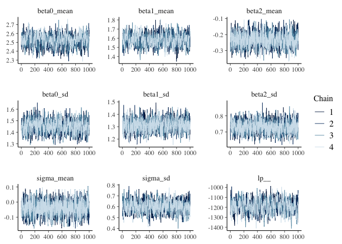
You can see from the output that there is only a small number divergent
transitions, which are rare enough that they shouldn’t pose any
challenges for interpreting the results (these can probably be further
reduced by increasing adapt_delta above it’s default value of 0.8).
There are also no more instances of the maximum treedepth being reached.
The summary statistics and traceplot of the population parameters show
the model has converged.
parameters = c("beta0_mean", "beta1_mean","beta2_mean", "beta0_sd", "beta1_sd","beta2_sd","sigma_mean","sigma_sd","lp__")

fit_ncs$summary(variables = parameters)
## # A tibble: 9 × 10
##   variable        mean   median      sd     mad       q5      q95  rhat ess_bulk
##   <chr>          <dbl>    <dbl>   <dbl>   <dbl>    <dbl>    <dbl> <dbl>    <dbl>
## 1 beta0_mean   2.52e+0  2.52e+0  0.0669  0.0661  2.41e+0  2.63e+0  1.01     535.
## 2 beta1_mean   1.58e+0  1.58e+0  0.0622  0.0606  1.48e+0  1.69e+0  1.00     564.
## 3 beta2_mean  -2.31e-1 -2.31e-1  0.0410  0.0406 -2.98e-1 -1.62e-1  1.00    1294.
## 4 beta0_sd     1.45e+0  1.45e+0  0.0514  0.0518  1.37e+0  1.53e+0  1.00     896.
## 5 beta1_sd     1.31e+0  1.31e+0  0.0474  0.0472  1.23e+0  1.39e+0  1.00    1051.
## 6 beta2_sd     7.32e-1  7.32e-1  0.0352  0.0358  6.76e-1  7.91e-1  1.00    1154.
## 7 sigma_mean  -4.14e-2 -4.18e-2  0.0448  0.0459 -1.15e-1  3.27e-2  1.00    1230.
## 8 sigma_sd     6.02e-1  6.03e-1  0.0508  0.0505  5.18e-1  6.85e-1  1.00     700.
## 9 lp__        -1.19e+3 -1.19e+3 63.1    63.4    -1.29e+3 -1.08e+3  1.01     427.
## # ℹ 1 more variable: ess_tail <dbl>
mcmc_trace(fit_ncs$draws(variables = parameters))
It’s also possible to apply non-centered transformations to double bounded parameters that have lower bounds and upper bounds (e.g., probability parameters that are constrained between 0 and 1). But there’s a bit more to think about with double bounded parameters, so I think I’ll address those in a future post. What I really want to get to in this post is how to apply non-centered transformations to multivariate distributions.
Non-Centered Parameterisation for Multivariate Distributions
The models presented above assume that individual variation in the
parameters are uncorrelated. In other words, knowing one person’s value
of beta0 gives us no information about their plausible beta1 and
beta2 values. However, in many cases, it’s reasonable to assume these
quantities are correlated. Returning to the example question of how the
number of hours we spend working affects our mental health, it’s
plausible that those with lower levels of mental health overall suffer
more from working longer hours. To examine this possibility, we need to
allow for the individual-specific parameters to be correlated. First,
let’s simulate some data where this is the case. The code below
simulates data from a model where beta0, beta1, and beta2 are
correlated, with Rho containing the parameter correlation matrix. In
principle, we could also allow the untransformed version of sigma to
also correlate with the beta parameters. But the transformation
applied to sigma makes the interpretation of this correlation less
straightforward. So we’ll keep it simple for now and assume sigma does
not correlate with the beta parameters.
# Set random seed for reproducibility
set.seed(123)

# Simulate data
N <- 2500  # Total number of observations
J <- 500    # Number of participants
n_j <- N / J  # Number of observations per participant

# Generate participant IDs and predictor variables
participant_id <- rep(1:J, each = n_j)
X1 <- rnorm(N, mean = 0, sd = 1)
X2 <- rnorm(N, mean = 0, sd = 1)

# Population parameter values
beta0_mean <- 2.5   # beta0 population mean
beta1_mean <- 1.5   # Effect of X1 population mean
beta2_mean <- -0.2  # Effect of X2 population mean
beta0_sd <- 1.5     # beta0 population SD
beta1_sd <- 1.3     # Effect of X1  population SD
beta2_sd <- 0.7     # Effect of X2 population SD
sigma_mean <- 0.7   # Residual mean
sigma_sd <- 0.3     # Residual SD

#Correlation matrix of individual parameters
Rho <- matrix(c(1,0.5,-0.5,
                0.5,1,0.4,
               -0.5,0.4,1),nrow=3,byrow=3)

#Diagonal matrix of population standard deviations
D <- diag(c(beta0_sd,beta1_sd,beta2_sd))

#Population covariance matrix
Sigma = D %*% Rho %*% D

#Vector of population means
Mu = c(beta0_mean,beta1_mean,beta2_mean)

# Generate correlated participant-specific parameters
theta <- MASS::mvrnorm(J, Mu, Sigma)

# Check correlation
cor(theta)
##            [,1]      [,2]       [,3]
## [1,]  1.0000000 0.4691356 -0.4676382
## [2,]  0.4691356 1.0000000  0.4564033
## [3,] -0.4676382 0.4564033  1.0000000
# Calculate participant-specific beta0s and slopes
beta0 <- theta[,1]
beta1 <- theta[,2]
beta2 <- theta[,3]

# Simulate variability in sigma
sigma <- rtruncnorm(n = N, a = 0, b = Inf, mean = sigma_mean, sd = sigma_sd)

# Generate response variable
Y <- rep(beta0, each = n_j) +
  rep(beta1, each = n_j) * X1 +
  rep(beta2, each = n_j) * X2 +
  rnorm(N, mean = 0, sd = rep(sigma, each = n_j))

# Prepare data for Stan
stan_data <- list(
  N = N,
  J = J,
  X1 = X1,
  X2 = X2,
  Y = Y,
  participant_id = participant_id
)
Let’s now tweak the model above to account for the covariation between
these parameters. As with the uncorrelated versions above, there are a
number of ways we can parameterise the model. In the version below, we
directly estimate population_cov, which is the population covariance
matrix of the individual-level parameters. The presence of this
covariance matrix increases the amount of information pooling the
happens when estimating the model. Whereas in the above models, a
participant’s estimate of a given parameter was constrained by other
participants’ estimates of that same parameter, now the estimate of
each beta parameter is influenced by other participants’ estimates of
not only that same parameter but also of estimates of the other beta
parameters. This extra pooling of information is especially helpful when
there are relatively few observations per individual. The prior
distribution of this covariance matrix is an inverse-wishart
distribution, a commonly used prior for estimating covariance matrices,
with 4 degrees of freedom and an identity scale matrix. The model also
includes a generated quantities block that converts the population
covariance matrix into a vector of population SDs and a population
correlation matrix.
stan_model_mv_cov <- "
data {
  int<lower=0> N;               // Number of observations
  int<lower=0> J;               // Number of participants
  vector[N] X1;                 // Predictor 1
  vector[N] X2;                 // Predictor 2
  vector[N] Y;                  // Response variable
  array[N] int participant_id;  // Participant IDs
}

parameters {
  vector[3] population_means;          // Population means for beta0, beta1, beta2
  cov_matrix[3] population_cov;        // Covariance matrix for beta0, beta1, and beta2
  array[J] vector[3] theta;            // Individual-level beta0, beta1, and beta2 estimates
  real sigma_mean;                     // Residual population mean (before transformation)
  real<lower=0> sigma_sd;              // Residual population SD (before transformation)
  vector[J] sigma_z;                   // Individual-level residuals (z-score, before transformation)
}

transformed parameters {
  vector[J] sigma = log1p_exp(sigma_mean + sigma_sd * sigma_z);
  vector[J] beta0 = to_vector(theta[,1]);
  vector[J] beta1 = to_vector(theta[,2]);
  vector[J] beta2 = to_vector(theta[,3]);
}

model {
  // Population-level priors
  population_means ~ normal(0, 5);
  population_cov ~ inv_wishart(4,identity_matrix(3));
  sigma_mean ~ normal(0, 2.5);
  sigma_sd ~ normal(0, 2.5);

  // Participant-level priors
  theta ~ multi_normal(population_means, population_cov);
  sigma_z ~ std_normal();

  // Likelihood
  Y ~ normal(beta0[participant_id] + beta1[participant_id] .* X1 + beta2[participant_id] .* X2, sigma[participant_id]);
}

generated quantities {
  //Convert population covariance matrix to population correlation matrix
  vector[3] population_sds = sqrt(diagonal(population_cov)); //extract variances and convert to SDs

  //The code below equates to: diag_matrix(population_sds)^-1 *  population_cov * diag_matrix(population_sds)^-1
  corr_matrix[3] population_corr = mdivide_right_spd(mdivide_left_spd(diag_matrix(population_sds),population_cov),diag_matrix(population_sds));
}"

# Compile the model
mod_mv_cov <- cmdstan_model(write_stan_file(stan_model_mv_cov))

# Fit the model
fit_mv_cov <- mod_mv_cov$sample(
  data = stan_data,
  seed = 123,
  chains = 4,
  parallel_chains = 4,
  refresh = 0,
  show_exceptions = FALSE
)
## Running MCMC with 4 parallel chains...
##
## Chain 2 finished in 41.2 seconds.
## Chain 3 finished in 47.3 seconds.
## Chain 1 finished in 52.4 seconds.
## Chain 4 finished in 54.9 seconds.
##
## All 4 chains finished successfully.
## Mean chain execution time: 49.0 seconds.
## Total execution time: 55.0 seconds.

## Warning: 6 of 4000 (0.0%) transitions ended with a divergence.
## See https://mc-stan.org/misc/warnings for details.
The model below shows another way to parameterise a model with
correlated individual-level parameters. This version decouples the
standard deviations of the population distributions from the
correlations. Separating the standard deviations from the correlations
in this way avoids the problem of the scale of the population
distributions influencing the degree of covariation between the
parameters, which can happen when the covariance matrix is directly
estimated. The major change in this model is that we separately estimate
population_corr which is the population correlation matrix of the
individual-level parameters and population_sds which is the standard
deviation of the population distributions. The code
quad_form_diag(population_corr, population_sds) converts the
correlation matrix and vector of SDs to a covariance matrix, which is
needed to compute the PDF of the multivariate normal distribution (this
is the opposite operation to what is done in the generated quantities
block of the model above). The prior distribution of this correlation
matrix is an LKJ distribution with a concentration parameter of 1, which
is a uniform prior across all possible correlation matrices.
stan_model_mv_cor <- "
data {
  int<lower=0> N;               // Number of observations
  int<lower=0> J;               // Number of participants
  vector[N] X1;                 // Predictor 1
  vector[N] X2;                 // Predictor 2
  vector[N] Y;                  // Response variable
  array[N] int participant_id;  // Participant IDs
}

parameters {
  vector[3] population_means;          // Population means for beta0, beta1, beta2
  vector<lower=0>[3] population_sds;   // Population SDs for beta0, beta1, beta2
  corr_matrix[3] population_corr;      // Correlation matrix for beta0, beta1, and beta2
  array[J] vector[3] theta;            // Individual-level beta0, beta1, and beta2 estimates
  real sigma_mean;                     // Residual population mean (before transformation)
  real<lower=0> sigma_sd;              // Residual population SD (before transformation)
  vector[J] sigma_z;                   // Individual-level residuals (z-score, before transformation)
}

transformed parameters {
  vector[J] sigma = log1p_exp(sigma_mean + sigma_sd * sigma_z);
  vector[J] beta0 = to_vector(theta[,1]);
  vector[J] beta1 = to_vector(theta[,2]);
  vector[J] beta2 = to_vector(theta[,3]);
}

model {
  // Population-level priors
  population_means ~ normal(0, 5);
  population_sds ~ normal(0, 2.5);
  population_corr ~ lkj_corr(1);
  sigma_mean ~ normal(0, 2.5);
  sigma_sd ~ normal(0, 2.5);

  // Participant-level priors
  theta ~ multi_normal(population_means, quad_form_diag(population_corr, population_sds));
  sigma_z ~ std_normal();

  // Likelihood
  Y ~ normal(beta0[participant_id] + beta1[participant_id] .* X1 + beta2[participant_id] .* X2, sigma[participant_id]);
}"

# Compile the model
mod_mv_cor <- cmdstan_model(write_stan_file(stan_model_mv_cor))

# Fit the model
fit_mv_cor <- mod_mv_cor$sample(
  data = stan_data,
  seed = 123,
  chains = 4,
  parallel_chains = 4,
  refresh = 0,
  show_exceptions = FALSE
)
## Running MCMC with 4 parallel chains...
##
## Chain 2 finished in 44.1 seconds.
## Chain 1 finished in 51.0 seconds.
## Chain 4 finished in 53.9 seconds.
## Chain 3 finished in 54.8 seconds.
##
## All 4 chains finished successfully.
## Mean chain execution time: 50.9 seconds.
## Total execution time: 54.8 seconds.

## Warning: 2 of 4000 (0.0%) transitions ended with a divergence.
## See https://mc-stan.org/misc/warnings for details.
Finally, the version below extends on the version above and implements a
non-centered version of this model. The first change here is that we’re
no longer estimating the correlation matrix. Instead, we’re estimating
the cholesky factor of the correlation matrix, which makes things
computationally simpler (we adopt the commonly used L_ notation to
denote cholesky factors here). Once we compute the cholesky factor of
the covariance matrix, we apply the multivariate version of the
inverse-z transform to compute the values of beta0, beta1, and
beta2. And then we can compute the likelihood in the same way we have
in the previous model. The model below also includes a
generated quantities block which converts the cholesky factor of the
population correlation matrix to the raw correlation matrix, so that
these correlations can be more easily interpreted.
stan_model_mv_cor_nc <- "
data {
  int<lower=0> N;               // Number of observations
  int<lower=0> J;               // Number of participants
  vector[N] X1;                 // Predictor 1
  vector[N] X2;                 // Predictor 2
  vector[N] Y;                  // Response variable
  array[N] int participant_id;  // Participant IDs
}

parameters {
  vector[3] population_means;                     // Population means for beta0, beta1, beta2
  vector<lower=0>[3] population_sds;              // Population SDs for beta0, beta1, beta2
  cholesky_factor_corr[3] L_population_corr;      // Cholesky factor of correlation matrix for beta0, beta1, and beta2
  matrix[J,3] theta_z;                            // Individual-level beta0, beta1, and beta2 estimates (z-score)
  real sigma_mean;                                // Residual population mean (before transformation)
  real<lower=0> sigma_sd;                         // Residual population SD (before transformation)
  vector[J] sigma_z;                              // Individual-level residuals (z-score, before transformation)
}

transformed parameters {
  vector[J] sigma = log1p_exp(sigma_mean + sigma_sd * sigma_z);
  matrix[3,3] L_population_cov = diag_pre_multiply(population_sds,L_population_corr);
  matrix[J,3] theta = rep_matrix(population_means',J) + theta_z * L_population_cov';
  vector[J] beta0 = theta[,1];
  vector[J] beta1 = theta[,2];
  vector[J] beta2 = theta[,3];
}

model {
  // Population-level priors
  population_means ~ normal(0, 5);
  population_sds ~ normal(0, 2.5);
  L_population_corr ~ lkj_corr_cholesky(1);
  sigma_mean ~ normal(0, 2.5);
  sigma_sd ~ normal(0, 2.5);

  // Participant-level priors
  to_vector(theta_z) ~ std_normal();
  sigma_z ~ std_normal();

  // Likelihood
  Y ~ normal(beta0[participant_id] + beta1[participant_id] .* X1 + beta2[participant_id] .* X2, sigma[participant_id]);
}

generated quantities {
  //Compute population correlation matrix from its cholesky factor
  corr_matrix[3] population_corr = multiply_lower_tri_self_transpose(L_population_corr);
}
"

# Compile the model
mod_mv_cor_nc <- cmdstan_model(write_stan_file(stan_model_mv_cor_nc))

# Fit the model
fit_mv_cor_nc <- mod_mv_cor_nc$sample(
  data = stan_data,
  seed = 123,
  chains = 4,
  parallel_chains = 4,
  refresh = 0,
  show_exceptions = FALSE
)
## Running MCMC with 4 parallel chains...
##
## Chain 2 finished in 29.9 seconds.
## Chain 1 finished in 30.1 seconds.
## Chain 4 finished in 32.9 seconds.
## Chain 3 finished in 33.0 seconds.
##
## All 4 chains finished successfully.
## Mean chain execution time: 31.5 seconds.
## Total execution time: 33.1 seconds.

## Warning: 5 of 4000 (0.0%) transitions ended with a divergence.
## See https://mc-stan.org/misc/warnings for details.
As can be seen from the output below, all three of these models produce roughly the same parameter estimates.
parameters = c("population_means","population_sds", "population_corr","sigma_mean","sigma_sd","lp__")

fit_mv_cov$summary(variables = parameters)
## # A tibble: 18 × 10
##    variable       mean   median      sd     mad       q5      q95  rhat ess_bulk
##    <chr>         <dbl>    <dbl>   <dbl>   <dbl>    <dbl>    <dbl> <dbl>    <dbl>
##  1 populatio…  2.53e+0  2.53e+0  0.0670  0.0662    2.42   2.64e+0  1.00    4358.
##  2 populatio…  1.46e+0  1.46e+0  0.0653  0.0649    1.35   1.57e+0  1.00    4017.
##  3 populatio… -2.01e-1 -2.01e-1  0.0380  0.0379   -0.264 -1.38e-1  1.00    2910.
##  4 populatio…  1.46e+0  1.45e+0  0.0483  0.0483    1.38   1.54e+0  1.00    4237.
##  5 populatio…  1.36e+0  1.36e+0  0.0481  0.0488    1.28   1.44e+0  1.00    3345.
##  6 populatio…  7.19e-1  7.18e-1  0.0314  0.0315    0.669  7.72e-1  1.00    1720.
##  7 populatio…  1   e+0  1   e+0  0       0         1      1   e+0 NA         NA
##  8 populatio…  4.71e-1  4.72e-1  0.0388  0.0388    0.406  5.34e-1  1.00    2828.
##  9 populatio… -4.42e-1 -4.43e-1  0.0444  0.0442   -0.514 -3.68e-1  1.00    2804.
## 10 populatio…  4.71e-1  4.72e-1  0.0388  0.0388    0.406  5.34e-1  1.00    2828.
## 11 populatio…  1   e+0  1   e+0  0       0         1      1   e+0 NA         NA
## 12 populatio…  4.71e-1  4.72e-1  0.0449  0.0443    0.397  5.43e-1  1.00    1878.
## 13 populatio… -4.42e-1 -4.43e-1  0.0444  0.0442   -0.514 -3.68e-1  1.00    2804.
## 14 populatio…  4.71e-1  4.72e-1  0.0449  0.0443    0.397  5.43e-1  1.00    1878.
## 15 populatio…  1   e+0  1   e+0  0       0         1      1   e+0 NA         NA
## 16 sigma_mean -6.27e-2 -6.20e-2  0.0419  0.0415   -0.133  3.95e-3  1.00    1351.
## 17 sigma_sd    5.90e-1  5.89e-1  0.0485  0.0476    0.509  6.72e-1  1.01     537.
## 18 lp__       -8.69e+2 -8.69e+2 55.6    54.5    -961.    -7.78e+2  1.01     438.
## # ℹ 1 more variable: ess_tail <dbl>
fit_mv_cor$summary(variables = parameters)
## # A tibble: 18 × 10
##    variable      mean   median      sd     mad       q5      q95   rhat ess_bulk
##    <chr>        <dbl>    <dbl>   <dbl>   <dbl>    <dbl>    <dbl>  <dbl>    <dbl>
##  1 populati…  2.53e+0  2.53e+0  0.0688  0.0707    2.42   2.65e+0  0.999    6244.
##  2 populati…  1.46e+0  1.46e+0  0.0638  0.0656    1.35   1.56e+0  1.00     5721.
##  3 populati… -2.02e-1 -2.01e-1  0.0380  0.0376   -0.265 -1.39e-1  1.00     3840.
##  4 populati…  1.46e+0  1.46e+0  0.0507  0.0513    1.38   1.55e+0  1.00     4881.
##  5 populati…  1.36e+0  1.36e+0  0.0499  0.0504    1.29   1.45e+0  1.00     4261.
##  6 populati…  7.17e-1  7.16e-1  0.0311  0.0303    0.667  7.69e-1  1.00     2063.
##  7 populati…  1   e+0  1   e+0  0       0         1      1   e+0 NA          NA
##  8 populati…  4.71e-1  4.72e-1  0.0399  0.0396    0.405  5.35e-1  1.00     4043.
##  9 populati… -4.49e-1 -4.50e-1  0.0446  0.0453   -0.520 -3.74e-1  1.00     2716.
## 10 populati…  4.71e-1  4.72e-1  0.0399  0.0396    0.405  5.35e-1  1.00     4043.
## 11 populati…  1   e+0  1   e+0  0       0         1      1   e+0 NA          NA
## 12 populati…  4.80e-1  4.82e-1  0.0441  0.0438    0.405  5.50e-1  1.00     2858.
## 13 populati… -4.49e-1 -4.50e-1  0.0446  0.0453   -0.520 -3.74e-1  1.00     2716.
## 14 populati…  4.80e-1  4.82e-1  0.0441  0.0438    0.405  5.50e-1  1.00     2858.
## 15 populati…  1   e+0  1   e+0  0       0         1      1   e+0 NA          NA
## 16 sigma_me… -5.50e-2 -5.50e-2  0.0417  0.0416   -0.124  1.45e-2  1.01     1193.
## 17 sigma_sd   5.93e-1  5.93e-1  0.0487  0.0494    0.515  6.74e-1  1.01      658.
## 18 lp__      -8.47e+2 -8.46e+2 60.6    59.1    -947.    -7.46e+2  1.01      429.
## # ℹ 1 more variable: ess_tail <dbl>
fit_mv_cor_nc$summary(variables = parameters)
## # A tibble: 18 × 10
##    variable       mean   median      sd     mad       q5      q95  rhat ess_bulk
##    <chr>         <dbl>    <dbl>   <dbl>   <dbl>    <dbl>    <dbl> <dbl>    <dbl>
##  1 populatio…  2.53e+0  2.53e+0  0.0656  0.0683  2.43e+0  2.64e+0  1.01     416.
##  2 populatio…  1.45e+0  1.45e+0  0.0648  0.0653  1.35e+0  1.56e+0  1.01     512.
##  3 populatio… -2.04e-1 -2.04e-1  0.0374  0.0371 -2.66e-1 -1.42e-1  1.00    1062.
##  4 populatio…  1.46e+0  1.46e+0  0.0489  0.0499  1.38e+0  1.54e+0  1.00    1027.
##  5 populatio…  1.36e+0  1.36e+0  0.0500  0.0507  1.29e+0  1.45e+0  1.00    1115.
##  6 populatio…  7.16e-1  7.16e-1  0.0322  0.0323  6.63e-1  7.71e-1  1.00    1303.
##  7 populatio…  1   e+0  1   e+0  0       0       1   e+0  1   e+0 NA         NA
##  8 populatio…  4.73e-1  4.73e-1  0.0388  0.0382  4.09e-1  5.36e-1  1.01     820.
##  9 populatio… -4.49e-1 -4.50e-1  0.0459  0.0455 -5.22e-1 -3.71e-1  1.00    1227.
## 10 populatio…  4.73e-1  4.73e-1  0.0388  0.0382  4.09e-1  5.36e-1  1.01     820.
## 11 populatio…  1   e+0  1   e+0  0       0       1   e+0  1   e+0 NA         NA
## 12 populatio…  4.79e-1  4.80e-1  0.0458  0.0460  4.03e-1  5.52e-1  1.00    1604.
## 13 populatio… -4.49e-1 -4.50e-1  0.0459  0.0455 -5.22e-1 -3.71e-1  1.00    1227.
## 14 populatio…  4.79e-1  4.80e-1  0.0458  0.0460  4.03e-1  5.52e-1  1.00    1604.
## 15 populatio…  1   e+0  1   e+0  0       0       1   e+0  1   e+0 NA         NA
## 16 sigma_mean -5.40e-2 -5.29e-2  0.0430  0.0422 -1.25e-1  1.47e-2  1.00    1086.
## 17 sigma_sd    5.89e-1  5.88e-1  0.0486  0.0500  5.10e-1  6.69e-1  1.01     710.
## 18 lp__       -1.17e+3 -1.17e+3 62.9    63.8    -1.27e+3 -1.07e+3  1.01     394.
## # ℹ 1 more variable: ess_tail <dbl>
None of these models had any issues with sampling efficiency when applied to these data, but notice that the non-centered version finished much more quickly. In other datasets or for higher-dimensional models, these three parameterisations might differ quite substantially in how efficiently they’re able to explore the posterior. So if one parameterisation isn’t quite working, try one of the others!
-
I realise there’s a departure from Australian english in writing ‘centered’ instead of ‘centred’, but the latter just looks strange to me. So I’ll use ‘centered’. ↩